Quickstart guide

Requirements

The pyslammer package is built on Python 3.12. Earlier versions of Python 3 may work, but have not been tested.

Installation using pip

Install pyslammer using pip from the Python Package Index (PyPI):

pip install pyslammer

Basic Usage

With pyslammer installed, basic usage involves the following steps: 1. Import the pyslammer module 2. Import a ground motion 3. Perform a rigid sliding block analysis 4. View results

Import the pyslammer module

The recommended ailas for pyslammer is slam:

import pyslammer as slam

This allows use of pyslammer features within your code with the short prefix slam.

The primary object type within pyslammer is the SlidingBlockAnalysis object. At a minimum any SlidingBlockAnalysis requires a yield acceleration for the slope (\(k_y\)) and an input ground motion. As basic example, consider a rigid sliding block analysis on a slope with a yield acceleration of \(0.2\) g.

Import a ground motion

A small number of sample ground motion records are included with pyslammer. We will use one of the sample ground motion records, but we expect most users will import their ground motions from external sources. To use any signal for a ground motion, pyslammer needs a 1-D array of acceleration in units of \(g\) and the signal timestep (in seconds). See The available sample ground motions can be viewed with:

motions = slam.sample_ground_motions() # Load all sample ground motions
for motion in motions:
    print(motion)

Morgan_Hill_1984_CYC-285
Nisqually_2001_UNR-058
Imperial_Valley_1979_BCR-230
Northridge_1994_PAC-175
Chi-Chi_1999_TCU068-090
Cape_Mendocino_1992_PET-090
Coalinga_1983_PVB-045
Mammoth_Lakes-2_1980_CVK-090
Kocaeli_1999_ATS-090
Nahanni_1985_NS1-280
Mammoth_Lakes-1_1980_CVK-090
Duzce_1999_375-090
Loma_Prieta_1989_HSP-000
Landers_1992_LCN-345
N_Palm_Springs_1986_WWT-180
Kobe_1995_TAK-090
Coyote_Lake_1979_G02-050
Northridge_1994_VSP-360

For this example, we will use theImperial_Valley_1979_BCR-230 motion.

gm = motions["Imperial_Valley_1979_BCR-230"]

The timestep and acceleration signal for the imported ground motion are gm.dt and gm.accel, respectively.

Perform a rigid sliding block analysis

With the imported ground motion, gm, and the assumed value of \(k_y\), we can perform a rigid sliding block analysis with pySLAMMER’s RigidAnalysis object. This simultaneously creates an instance of RigidAnalysis and performs the analysis, which is stored as result. The inputs for RigidAnalysis are the input acceleration signal, time step, and the yield acceleration.

A note admonition! Not for anyting in particular, though...

ky = 0.2 # yield acceleration in g
result = slam.RigidAnalysis(ky, gm.accel, gm.dt)

View results

The primary output of the sliding block analysis is the final displacement (SlidingBlockAnalysis.max_sliding_disp). By default, all lengths in pySLAMMER are in meters. The cell below shows the displacement induced by the sample ground motion in the example:

print(f"Slope yield acc: {ky:.2f} g \nGround motion: {gm.name}; PGA: {gm.pga:.2f} g \nSliding displacement: {result.max_sliding_disp:.3f} m")

Slope yield acc: 0.20 g 
Ground motion: Imperial_Valley_1979_BCR-230; PGA: 0.77 g 
Sliding displacement: 0.213 m

A built-in plotting function presents an at-a-glance picture of the analysis result in terms of the input motion and block accelerations, sliding velocity, and sliding displacement:

fig = result.sliding_block_plot()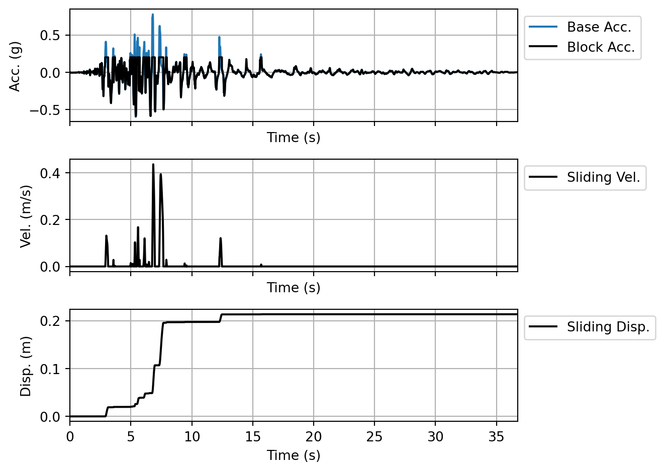

In addition to the final displacement, the displacement, velocity, and acceleration time histories of the block are returned as numpy arrays. See the documentation for the SlidingBlockAnalysis class for a detailed description of all the results.