import itertools
from dataclasses import dataclass
from pathlib import Path

import numpy as np
import pandas as pd
import matplotlib.pyplot as plt
from matplotlib.lines import Line2D
from matplotlib.legend_handler import HandlerTuple
from matplotlib.patches import FancyArrowPatch

import pyslammer as slam

plt.style.use(slam.psfigstyle)Performance-based seismic design for two highway segments
This example reproduces the illustrative performance-based seismic design (PBSD) study from the pySLAMMER software paper (Arnold and Garcia-Rivas 2026), in which a state highway agency assesses the seismic vulnerability of two road segments adjacent to slopes. It is the canonical example of pySLAMMER’s intended use: repeated coupled sliding-block analyses inside a probabilistic framework, the sort of workflow that is impractical with SLAMMER’s GUI.
For the full background and discussion, see §3 of the SoftwareX manuscript.
Runtime
The Monte Carlo loop below runs ~5,600 coupled analyses and takes roughly 15–30 minutes on a modern laptop. Results are cached to docs/_static/cache/pbsd_segments.pkl.gz after the first run; subsequent renders load the cache and are nearly instant. Delete the cache file to force a rerun.
Scenario
A state agency has a suite of design ground motions with a 5% probability of exceedance in 50 years and a damage model relating coupled sliding-block displacement, \(D\), to physical damage on bridges adjacent to slopes. A 25 cm displacement threshold corresponds to severe damage; the agency’s resilience target is that any segment with \(P(D > 25\,\text{cm})\) above 10% is “unacceptable” on critical routes.
Two road segments — A and B — sit adjacent to similar slopes. Segment A’s slope is moderately weaker and softer than Segment B’s. Uncertainty in slope strength (\(k_y\)) and stiffness (\(V_s\)) is captured as log-normal distributions; pySLAMMER is run repeatedly with parameter samples from those distributions until the relative standard error of the mean displacement falls below 5%.
| Parameter | Segment A | Segment B |
|---|---|---|
| Mean yield acceleration, \(\mu_{k_y}\) (g) | 0.13 | 0.15 |
| Mean shear-wave velocity, \(\mu_{V_s}\) (m/s) | 250 | 400 |
| \(\sigma_{\ln,k_y}\) | 0.2 | 0.2 |
| \(\sigma_{\ln,V_s}\) | 0.15 | 0.15 |
| Base shear-wave velocity, \(V_b\) (m/s) | 1500 | 1500 |
| Damping ratio | 0.05 | 0.05 |
| Reference strain | 0.0005 | 0.0005 |
| Slope height, \(H\) (m) | 25 | 25 |
Setup
A subset of pySLAMMER’s bundled motion suite is used as a stand-in for the agency’s design motion set. Each motion is scaled to a target PGA of 0.44 g.
record_names = [
    "Nisqually_2001_UNR-058",
    "Imperial_Valley_1979_BCR-230",
    "Northridge_1994_PAC-175",
    "Cape_Mendocino_1992_PET-090",
    "Coalinga_1983_PVB-045",
    "Mammoth_Lakes-1_1980_CVK-090",
    "Loma_Prieta_1989_HSP-000",
    "Coyote_Lake_1979_G02-050",
    "Northridge_1994_VSP-360",
]
histories = {k: v for k, v in slam.sample_ground_motions().items() if k in record_names}
print(f"{len(histories)} motions selected")
9 motions selectedSlope and analysis definitions
@dataclass
class Segment:
    name: str
    height: float
    ky_mean: float
    ky_cv: float
    vs_mean: float
    vs_cv: float
    vs_base: float


ky_cv = 0.2
vs_cv = 0.15
A = Segment("A", 25, 0.13, ky_cv, 250, vs_cv, 1500)
B = Segment("B", 25, 0.15, ky_cv, 400, vs_cv, 1500)


def run_coupled(ky, vs_slope, motion_name, gm, segment):
    """Run one coupled analysis at the given (ky, vs_slope) sample."""
    result = slam.Coupled(
        ky=ky,
        ground_motion=gm,
        target_pga=0.44,
        height=segment.height,
        vs_slope=vs_slope,
        vs_base=segment.vs_base,
        damp_ratio=0.05,
        ref_strain=0.0005,
        soil_model="equivalent_linear",
    )
    return {
        "segment": segment.name,
        "motion": motion_name,
        "ky": ky,
        "vs_slope": vs_slope,
        "k_max": float(np.max(result.a_in)),
        "d_max": float(result.max_sliding_disp),
    }
Monte Carlo sampling
The Monte Carlo loop draws \(k_y\) and \(V_s\) from log-normal distributions parameterized by each segment’s mean and coefficient of variation, runs a coupled analysis for every motion in the suite, and tracks the relative standard error of the mean displacement until it falls below 5% (or a hard cap of 700 outer iterations is reached).
Results are cached to disk on first run.
cache_path = Path("..") / "_static" / "cache" / "pbsd_segments.pkl.gz"

if cache_path.exists():
    df = pd.read_pickle(cache_path)
    print(f"Loaded {len(df)} rows from {cache_path}")
else:
    rng = np.random.default_rng(seed=42)
    target_rmse = 0.05
    runs = 700
    interval = 5

    all_results = []
    for segment in [A, B]:
        results = []
        ky_std = segment.ky_mean * segment.ky_cv
        vs_std = segment.vs_mean * segment.vs_cv
        ky_mu_ln = np.log(segment.ky_mean ** 2 / np.sqrt(ky_std ** 2 + segment.ky_mean ** 2))
        ky_sigma_ln = np.sqrt(np.log(1 + (ky_std / segment.ky_mean) ** 2))
        vs_mu_ln = np.log(segment.vs_mean ** 2 / np.sqrt(vs_std ** 2 + segment.vs_mean ** 2))
        vs_sigma_ln = np.sqrt(np.log(1 + (vs_std / segment.vs_mean) ** 2))

        for run in range(runs):
            for motion_name, gm in histories.items():
                ky = max(0.01, rng.lognormal(ky_mu_ln, ky_sigma_ln))
                vs_slope = max(0.01, rng.lognormal(vs_mu_ln, vs_sigma_ln))
                results.append(run_coupled(ky, vs_slope, motion_name, gm, segment))

            if (run + 1) % interval == 0:
                d = pd.DataFrame(results)["d_max"]
                rel_se = (d.std() / np.sqrt(len(d))) / d.mean()
                if rel_se < target_rmse:
                    print(f"Segment {segment.name}: converged at n={len(results)} (rel SE = {rel_se:.4f})")
                    break

        all_results.extend(results)

    df = pd.DataFrame(all_results)
    cache_path.parent.mkdir(parents=True, exist_ok=True)
    df.to_pickle(cache_path)
    print(f"Wrote {len(df)} rows to {cache_path}")
Segment A: converged at n=1260 (rel SE = 0.0495)
Segment B: converged at n=405 (rel SE = 0.0485)
Wrote 1665 rows to ../_static/cache/pbsd_segments.pkl.gzProbability of exceedance
The empirical probability of exceedance for each segment is computed by sorting the displacement samples and plotting the complementary cumulative distribution. The probability of exceeding 25 cm is read off the curve.
Code
def find_crossing_point(x_data, y_data, x_threshold):
    x_sorted_idx = np.argsort(x_data)
    x_sorted = np.asarray(x_data)[x_sorted_idx]
    y_sorted = np.asarray(y_data)[x_sorted_idx]
    if x_threshold < x_sorted.min() or x_threshold > x_sorted.max():
        return None
    return x_threshold, float(np.interp(x_threshold, x_sorted, y_sorted))


def prob_label(ax, x_rel, y_rel, segment, threshold, prob):
    ax.text(
        x_rel, y_rel,
        f"$P(D_{segment} >$ {100 * threshold:.0f} cm$)$\n = {100 * prob:.0f}%",
        transform=ax.transAxes,
        fontsize=10,
        verticalalignment="top",
        bbox=dict(facecolor="white", alpha=1),
        zorder=10,
    )


threshold = 0.25  # 25 cm severe-damage threshold
colors = {"A": "#1b9e77", "B": "#d95f02"}
markers = {"A": "o", "B": "^"}
label_location = {"A": (0.05, 0.13), "B": (0.69, 0.6)}

fig, ax = plt.subplots(figsize=(5, 4))
ax2 = ax.twinx()

legend_pairs = []
for segment in [A, B]:
    df_seg = df[df["segment"] == segment.name]
    sorted_d = np.sort(df_seg["d_max"])
    poe = 1 - np.arange(1, len(sorted_d) + 1) / len(sorted_d)

    line, = ax.plot(
        sorted_d, poe,
        color=colors[segment.name],
        linewidth=2,
        label=f"Segment {segment.name}",
    )
    crossing = find_crossing_point(sorted_d, poe, threshold)
    if crossing is not None:
        edpx, edpy = crossing
        ax.scatter(edpx, edpy, marker="o", s=75, facecolors="none",
                   edgecolors="black", linewidths=1.5, zorder=5)
        lx, ly = label_location[segment.name]
        prob_label(ax2, lx, ly, segment.name, edpx, edpy)

    scatter = ax2.scatter(
        df_seg["d_max"], df_seg["ky"],
        c=colors[segment.name],
        marker=markers[segment.name],
        alpha=0.4,
        s=5,
        zorder=2,
    )

    marker_proxy = Line2D([0], [0], marker=markers[segment.name], markersize=5,
                          markerfacecolor=colors[segment.name],
                          markeredgecolor=colors[segment.name],
                          alpha=0.5, linestyle="None")
    legend_pairs.append((line, marker_proxy))

ax.axvline(threshold, color="k", linewidth=1)
ax.set_xlabel("Coupled sliding block displacement, $D$ (m)")
ax.set_ylabel("Probability of exceedance")
ax.set_xscale("log")
ax.set_xlim(0.005, 2)
ax.set_ylim(0, 1)
ax.set_yticks(np.linspace(0, 1, 11))
ax.grid(which="both", linestyle=":", color="#d9d9d9")

ax2.set_ylim(0.05, 0.3)
ax2.set_ylabel("Yield acceleration, $k_y$ (g)")

ax.legend(
    legend_pairs,
    [f"Segment {seg.name}" for seg in [A, B]],
    handler_map={tuple: HandlerTuple(ndivide=None, pad=1)},
    handlelength=5,
    loc="upper right",
    bbox_to_anchor=(1.01, 1.012),
    borderpad=0.6,
)

plt.tight_layout()
plt.show()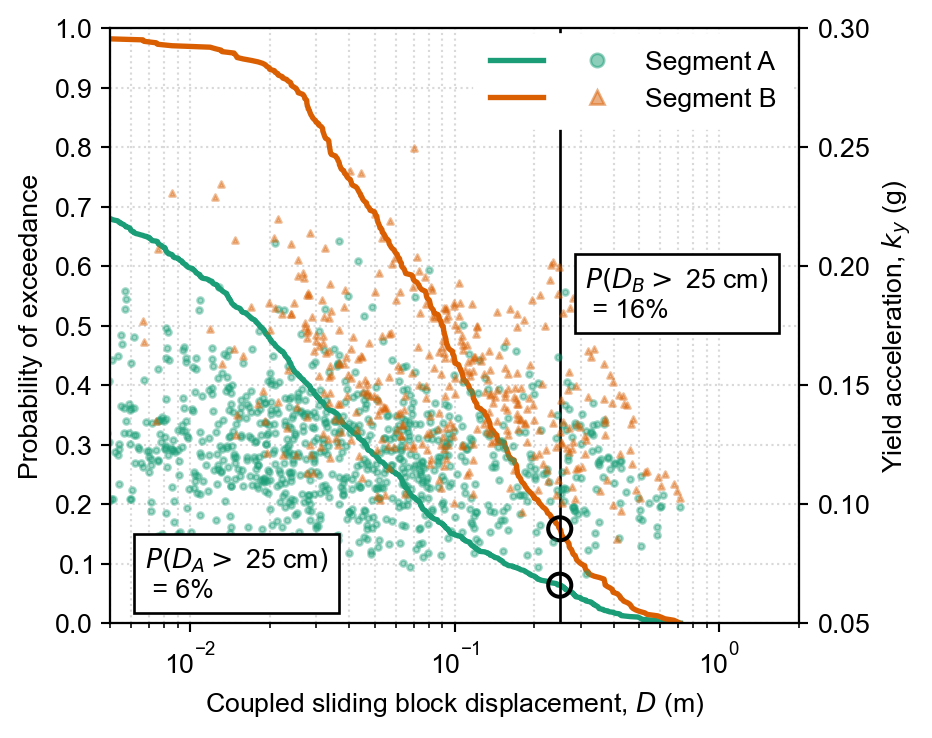
Discussion
The result is the headline finding from (Arnold and Garcia-Rivas 2026): despite Segment B having a higher mean yield acceleration, its probability of exceeding the 25 cm severe-damage threshold is roughly double Segment A’s. The counterintuitive behavior reflects the coupled response of the softer slope at Segment A — which would be missed by a rigid (Newmark) analysis. With the study’s results in hand, the agency can prioritize investment (further investigation, retrofit, or alternate routing) on Segment B rather than spreading resources across both.
The full discussion of the framework, the scaling to regional studies, and the broader case for performance-based seismic design as a pySLAMMER use case is in §3 of the manuscript.
References
Arnold, Lorne, and Andres Garcia-Rivas. 2026. “pySLAMMER: A Python Package for Sliding Block Analysis of Earthquake-Induced Landslides.” SoftwareX.