PySLAMMER’s rigid, decoupled, and coupled analysis methods are intended to produce sliding block analysis results that match the legacy SLAMMER results. This is an important feature for sliding block displacements, which are used as a performance index (as opposed to providing a direct prediction of actual slope displacement) in practice. Equivalence with legacy results allows new results to be interpreted with reference to historical analyses and experience.
Approach
To demonstrate pySLAMMER’s equivalence to SLAMMER, we performed several sliding block analyses across a broad parametric space. The three main categories of parameters studied were ground motion, analysis method, and analysis options.
Ground motion
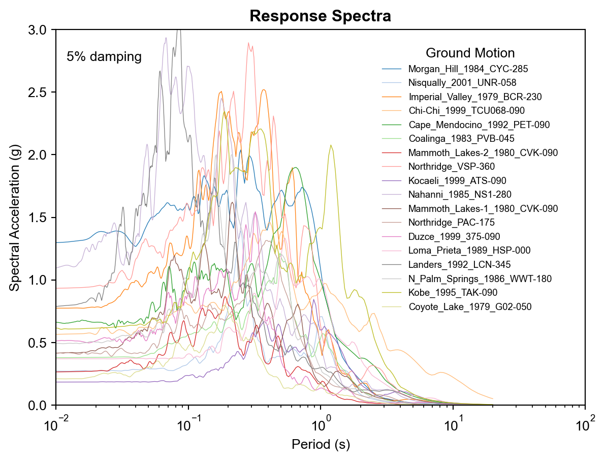
We used the motions from pySLAMMER’s built-in sample ground motion suite at several scales to capture a reasonable breadth of the familiar key engineering ground motion characteristics (frequency, amplitude, and duration). The acceleration response spectra for the input motion suite are shown in Figure 1. Additional details on the ground motions are provided on the ground motion suite page.
Code
# Navigate to ground motion suite response spectra filescurrent_dir = os.getcwd()folder_path = Path(current_dir).resolve() /"pySLAMMER_suite_resp"csv_files =list(folder_path.glob("*.csv"))# Read each CSV file into a DataFrame and store them in a listfreq_index =0resp_index =1spectra = {}for csv_file in csv_files: data = np.loadtxt(csv_file, delimiter=",", skiprows=2)# convert response from cm/s^2 to g's data[:, resp_index] = data[:, resp_index] /981 spectra[csv_file.name.strip(".csv")] = data# Initialize the plotfig, ax = plt.subplots()ax.set_prop_cycle(cycler(color=plt.cm.tab20.colors))for motion in spectra: ax.plot(1/spectra[motion][:, freq_index], spectra[motion][:, resp_index], label=motion, linewidth=0.5, )ax.text(0.012, 2.75, "5% damping")# Add labels, legend, and gridax.set_xlabel("Period (s)")ax.set_ylabel("Spectral Acceleration (g)")ax.set_title("Response Spectra")ax.set_xscale("log")ax.set_ylim(0,3)ax.set_xlim(0.01,100)ax.legend( loc="center left", bbox_to_anchor=(0.6, 0.6), fontsize="x-small", title="Ground Motion", title_fontsize="medium", frameon=False)plt.show()
Figure 1: Acceleration response spectra for input ground motions
Analysis methods
The three rigorous analysis methods that SLAMMER performs are the Rigid, Decoupled, and Coupled methods. Each of these methods, which are briefly described below, are implemented in pySLAMMER and included in this comparison.
Rigid Block Analysis
Conceptualized by Whitman in 1963 and further developed by Newmark in 1965 (Marcuson (1994), Newmark (1965)), rigid block analysis models a potential landslide mass as a rigid mass on an inclined plane base with a perfectly plastic frictional interface. The rigid block motion matches the base motion exactly until the acceleration of the base exceeds some critical value (the yield acceleration, \(k_y\)). Once this critical \(k_y\) value is reached, the block’s acceleration remains constant \(k_y\), resulting in relative velocity and displacement between block and base. The relative velocity is calculated by integrating the difference between the block and base accelerations. The displacement accumulated by the block moving down the ramp is calculated by integrating the relative velocity. Sliding stops (i.e., block motion again matches base motion exactly) when the relative velocity reaches zero.
Decoupled Analysis
Landslide materials are, of course, not rigid. Except for very shallow, stiff slide masses, the rigid block model does a poor job of approximating the dynamics of a co-seismic landslide system. The decoupled method was developed to provide some way of accounting for the deformation of the slope mass due to shaking (Seed and Martin (1966), Makdisi and Seed (1978)) . It consists of two distinct (or decoupled, if you will) calculations: dynamic response and rigid sliding. During the dynamic response phase, the possibility of sliding is ignored while the slope response to strong ground motion is calculated. The average internal acceleration of the slope mass during this first phase is then used as the base input acceleration for the second phase (rigid sliding) which is simply a rigid block analysis.
Coupled Analysis
As indicated by the name, coupled analysis takes the two separate calculations from the decoupled analysis and performs them simultaneously. Chopra and Zhang (1991) introduced a coupled sliding block method for concrete gravity dams that considers the dam as a distributed mass system. Kramer and Smith (1997) developed a coupled analysis method for soil slopes using discrete masses. Rathje and Bray (1999) modified Chopra and Zhang’s distributed mass approach and applied it to earth structures. The coupled method used by SLAMMER (and pySLAMMER) is Rathje and Bray’s modification of Chopra and Zhang. With coupled sliding, the sliding mass’s dynamic response is calculated for both sliding and non-sliding conditions. Sliding stops when the relative velocity of the sliding mass reaches zero. The stop of sliding can introduce an abrupt change in acceleration applied to the sliding mass. Because the dynamic response is being calculated continually through the analysis, the approach to identifying the timing of these abrupt changes will affect potential subsequent sliding events.
Dynamic Response
The Decoupled and Coupled methods both require the calculation of the slope’s dynamic response. The two methods for dynamic response in SLAMMER, which have been carried over to pySLAMMER are linear elastic and equivalent linear.
Analysis options
SLAMMER allows users to include a constant \(k_y\) value or a variable \(k_y\) that changes with accumulated sliding displacement. The \(k_y\) – displacement relationship is stepwise with a table of paired values. This feature provides a rough means of approximating post-peak residual strength. 1
The dynamic response of the system (applicable to decoupled and coupled analyses) is calculated using either linear elastic or equivalent linear assumptions. The minimum input parameters needed for the linear elastic analyses are a damping ration, the slope height, and the shear wave velocity of the material above and below the slip surface. For equivalent linear analysis, a reference strain parameter is also needed. Although not explicitly documented, inspection of the SLAMMER source code uses Darendeli (2001) modulus reduction and damping curves with a curvature coefficient of 1.
Separate entries for the shear wave velocity of the material above and below the slip surface (\(V_s\) and \(V_b\), respectively) are used to introduce an equivalent foundation radiation damping into the viscous material damping as described by Lee (2004). This happens behind the scenes in SLAMMER by default and cannot be turned off. 2
Table 1 shows the analysis options and ranges of input values used in the group of simulations used to compare pySLAMMER to
Code
kykmax = [0.05, 1.0]tmts = [0.1, 10.0]height = [0.1, 100]vs = [200, 1200]vsvb = [0.1, 100]damp = [5, 25]ref_str = [1, 10]params = {"param": ["Methods","Dynamic Resp.","ky/kmax","Tm/Tx *","Slope height (m) *","Slope shear wave vel., Vs (m/s) *","Vs/Vb *","Damping (%) *","Reference strain (%) **" ],"val": ["Rigid, Decoupled, Coupled","Linear elastic, Equivalent linear",f"{kykmax[0]} to {kykmax[1]}",f"{tmts[0]} to {tmts[1]}",f"{height[0]} to {height[1]}",f"{vs[0]} to {vs[1]}",f"{vsvb[0]} to {vsvb[1]}",f"{damp[0]} to {damp[1]}",f"{ref_str[0]} to {ref_str[1]}" ]}# * only applicable to Decoupled and Coupled methods# ** only applicable to equivalent linear dynamic responsetbl = ( GT(pd.DataFrame(params)) .cols_label( param=html("Parameter"), val=html("Range / Options used") ) .cols_align(align="center", columns=1) .tab_source_note("* Only applies to Decouled and Coupled analyses") .tab_source_note("** Only applies to equivalent linear analyses"))tbl
Table 1: Sliding block parameters used for pySLAMMER to SLAMMER comparison analyses.
Parameter
Range / Options used
Methods
Rigid, Decoupled, Coupled
Dynamic Resp.
Linear elastic, Equivalent linear
ky/kmax
0.05 to 1.0
Tm/Tx *
0.1 to 10.0
Slope height (m) *
0.1 to 100
Slope shear wave vel., Vs (m/s) *
200 to 1200
Vs/Vb *
0.1 to 100
Damping (%) *
5 to 25
Reference strain (%) **
1 to 10
* Only applies to Decouled and Coupled analyses
** Only applies to equivalent linear analyses
Equivalence criteria
Although the Python code in pySLAMMER essentially uses the same algorithms as the Java code in SLAMMER, minor numerical differences should be expected due to implementation details (e.g., number type handling, order of operations) (Ince, Hatton, and Graham-Cumming 2012). However, the results can be considered functionally equivalent if they contain no diverging tendencies and the differences are relatively small. For engineering purposes, sliding block displacements below 0.5 cm can be considered equivalent to zero displacement (Bray and Macedo 2019).
The thresholds used to determine functional equivalence are based on linear regression of results between the two programs and absolute differences of individual analysis pairs. Table 2 shows these criteria.
Code
equiv_data = {"criterion": ["Relative error","Absolute error","Small displacement threshold *","Small disp. absolute error *","Individual tests passing","Linear regression slope","Linear regression intercept","Linear regression R²", ],"threshold": ["± 2%","± 1.0 cm","0.5 cm","± 0.05 cm","≥ 95%","1 ± 0.01","0 ± 0.1 cm","≥ 0.99", ],"category": ["Individual","Individual","Individual","Individual","Group","Group","Group","Group", ]}equiv_df = pd.DataFrame(equiv_data)tbl_equiv = ( GT(equiv_df, groupname_col="category") .cols_label( criterion=html("Criterion"), threshold=html("Threshold"), ) .cols_align(align="center", columns="threshold") .tab_source_note("* For displacements below threshold, only absolute error criterion applies") .tab_source_note("Individual test tolerances are enforced in aggregate by the group pass rate"))tbl_equiv
Table 2: Equivalence criteria for pySLAMMER verification against SLAMMER.
Criterion
Threshold
Individual
Relative error
± 2%
Absolute error
± 1.0 cm
Small displacement threshold *
0.5 cm
Small disp. absolute error *
± 0.05 cm
Group
Individual tests passing
≥ 95%
Linear regression slope
1 ± 0.01
Linear regression intercept
0 ± 0.1 cm
Linear regression R²
≥ 0.99
* For displacements below threshold, only absolute error criterion applies
Individual test tolerances are enforced in aggregate by the group pass rate
Results
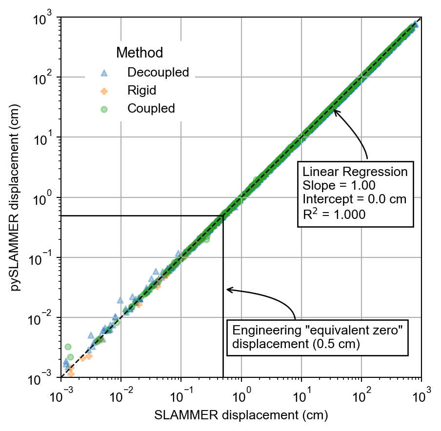
The results of the simulations across the parametric space described in Table 1 are shown on Figure 2. The data are plotted on a log-log scale to make minor numerical differences visible near and below the “equivalent zero” displacement threshold. As indicated by the linear regression statistics, the differences between SLAMMER and pySLAMMER results are negligibly small relative to scales of engineering significance.
Code
# Load SLAMMER and pySLAMMER results from verification data# Load SLAMMER results tests/verification_data/results/slammer_results.json.gzslammer_path = project_root /"tests"/"verification_data"/"results"/"slammer_results.json.gz"with gzip.open(slammer_path, 'rt') as f: slammer_data = json.load(f)# Load pySLAMMER results pyslammer_path = project_root /"tests"/"verification_data"/"results"/"pyslammer_0.2.3_results.json.gz"with gzip.open(pyslammer_path, 'rt') as f: pyslammer_data = json.load(f)# Create comparison dataframecomparison_data = []# Create lookup for pySLAMMER results by analysis_idpyslammer_lookup = {analysis['analysis_id']: analysis for analysis in pyslammer_data['analyses']}for slammer_analysis in slammer_data['analyses']: analysis_id = slammer_analysis['analysis_id']if analysis_id in pyslammer_lookup: pyslammer_analysis = pyslammer_lookup[analysis_id]# Get method name and convert to title case method = slammer_analysis['analysis']['method'] method_name = method.title() if method !='rigid'else'Rigid' comparison_data.append({'analysis_id': analysis_id,'Method': method_name,'SLAMMER': slammer_analysis['results']['normal_displacement_cm'],'pySLAMMER': pyslammer_analysis['results']['normal_displacement_cm'] })# Create dataframedfp = pd.DataFrame(comparison_data)# Calculate overall linear regression for statistics displayfrom scipy.stats import linregressslope, intercept, r, p, se = linregress(dfp['SLAMMER'], dfp['pySLAMMER'])plt.close("all")############# pySLAMMER v. SLAMMER############plt.rcParams["font.family"] ="Arial"plt.rcParams["font.sans-serif"] = ["Arial"]plt.rcParams["savefig.dpi"] =600fig, ax = plt.subplots()keys = ["Decoupled", "Rigid", "Coupled"]markers = ["^", "P", "o"]for i, key inenumerate(keys): grp = dfp[dfp["Method"] == key] ax.scatter(grp["SLAMMER"], grp["pySLAMMER"], label=key, alpha=0.35, marker=markers[i], s=20 )ax.set_xscale("log")ax.set_yscale("log")ax.set_xlim(1e-3, 1e3)ax.set_ylim(1e-3, 1e3)ax.set_aspect("equal")plt.grid()ax.set_xlabel("SLAMMER displacement (cm)")ax.set_ylabel("pySLAMMER displacement (cm)")# Linear regressionax.plot([1e-3, 1e3], [1e-3, 1e3], color="black", linestyle="--", linewidth=1)ax.text(0.67,0.585,f"Linear Regression\nSlope = {slope:.2f}\nIntercept = {intercept:.1f} cm\nR$^2$ = {r**2:.3f}", transform=ax.transAxes, fontsize=10, verticalalignment="top", bbox=dict(facecolor="white", alpha=1),)# Arrow for linear regressionarrow = FancyArrowPatch( (0.85, 0.6), # Start point (near text box) (0.75, 0.75), # End point (middle of plot, on dashed line) connectionstyle="angle3,angleA=90,angleB=-45", # Angle connection style transform=ax.transAxes, arrowstyle="->", mutation_scale=11, color="black", alpha=1, zorder=4)ax.add_patch(arrow)# Engineering range of interestax.plot([0,0.5,0.5],[0.5,0.5,0], color="black", linestyle="-", linewidth=1)# Add text box with regression statisticsax.text(0.475,0.145,"Engineering \"equivalent zero\"\ndisplacement (0.5 cm)", transform=ax.transAxes, fontsize=10, verticalalignment="top", bbox=dict(facecolor="white", alpha=1),)# Arrow for linear regressionarrow = FancyArrowPatch( (0.65, 0.155), # Start point (near text box) (0.45, 0.245), # End point (middle of plot, on dashed line) connectionstyle="angle3,angleA=90,angleB=-5", # Angle connection style transform=ax.transAxes, arrowstyle="->", mutation_scale=10, color="black", alpha=1, zorder=4,)ax.add_patch(arrow)# Add legendax.legend( loc="upper left", bbox_to_anchor=(0.05, 0.95), fontsize=10, title="Method", title_fontsize="11", framealpha=1,)plt.show()
Figure 2: Comparison of pySLAMMER and SLAMMER analysis results. At this scale, the differences are too small to be distinguished visually.
The equivalence check against the criteria in Table 2 is implemented through automated pre-release testing in pySLAMMER. All three methods (rigid, decoupled, and coupled) passed all equivalence criteria. The full verification report for the current release (v0.2.3) is available in the pySLAMMER repository. Reports for all released versions can be browsed in the verification results directory.
Conclusions
The results show that pySLAMMER is performing the same rigorous analysis methods as SLAMMER. Across a broad array of input parameters, the results are identical or nearly identical against the equivalence criteria in Table 2. Minor numerical differences between the output of the two programs are to be expected. However, the differences are so small as to be insignificant for engineering purposes, both in research and practice.
References
Bray, Jonathan D., and Jorge Macedo. 2019. “Procedure for Estimating Shear-Induced Seismic Slope Displacement for Shallow Crustal Earthquakes.”Journal of Geotechnical and Geoenvironmental Engineering 145 (12): 04019106. https://doi.org/10.1061/(ASCE)GT.1943-5606.0002143.
Ince, Darrel C., Leslie Hatton, and John Graham-Cumming. 2012. “The Case for Open Computer Programs.”Nature 482 (7386): 485–88. https://doi.org/10.1038/nature10836.
Kramer, Steven L, and Matthew W Smith. 1997. “Modified Newmark Model for Seismic Displacements of Compliant Slopes.”Journal of Geotechnical and Geoenvironmental Engineering 123 (7).
Makdisi, Faiz I., and H. Bolton Seed. 1978. “Simplified Procedure for Estimating Dam and Embankment Earthquake-Induced Deformations.”Journal of the Geotechnical Engineering Division 104 (7): 849–67. https://doi.org/10.1061/AJGEB6.0000668.
Marcuson, W. 1994. “A Symposium in Honor of Robert v. Whitman.” In.
Newmark, N. M. 1965. “Effects of Earthquakes on Dams and Embankments.”Geotechnique 15 (2): 139–60.
Rathje, E. M., and J. D. Bray. 1999. “An Examination of Simplified Earthquake-Induced Displacement Procedures for Earth Structures.”Canadian Geotechnical Journal 36 (1): 72–87. https://doi.org/10.1139/cgj-36-1-72.
Seed, H. Bolton, and Geoffrey R. Martin. 1966. “The Seismic Coefficient in Earth Dam Design.”Journal of the Soil Mechanics and Foundations Division 92 (3): 25–58. https://doi.org/10.1061/JSFEAQ.0000871.
Footnotes
pySLAMMER includes additional options for variable yield acceleration, but only stepwise variation is applicable to comparison with SLAMMER↩︎
If lower total damping than the equivalent foundation radiation damping is needed for some reason (e.g., for comparison with published analyses that did not include this damping mechanism) both SLAMMER and pySLAMMER accept negative values for damping ratio, which can be used to offset the damping applied by the foundation radiation damping.↩︎