import pyslammer as slamBatch Simulations
This notebook shows an example use case of pyslammer for running batch simulations.
Setup
The next steps assume you’ve already installed pySLAMMER from PYPI. See the quickstart guide for installation instructions.
Import pyslammer using:
Additional Python libraries, such as matplotlib may also be useful.
import numpy as np
import pandas as pd
import matplotlib.pyplot as plt
plt.style.use(slam.psfigstyle)
kys = np.linspace(0.01,0.7,100)
histories = slam.sample_ground_motions()
output = {}Batch Simulations
The code below evaluates all combinations of \(k_y\) contained in kys and every motion in histories. Some key features (motion, ky, max displacement, and displacement time histories) are stored in a dictionary, which is then converted to a pandas dataframe.
run = 0
for ky in kys:
    for motion, hist in histories.items():
        result = slam.RigidAnalysis(ky,histories[motion].accel, histories[motion].dt,target_pga=0.3)
        output[run] = {"motion":motion, "ky":ky, "k_max":np.max(result.a_in), "d_max": result.max_sliding_disp, "dt":result.dt, "disp": result
        .sliding_disp}
        run += 1
# convert the output to a pandas dataframe
df = pd.DataFrame.from_dict(output,orient='index')
df| motion | ky | k_max | d_max | dt | disp | |
|---|---|---|---|---|---|---|
| 0 | Morgan_Hill_1984_CYC-285 | 0.01 | 0.112099 | 1.539165e-01 | 0.005 | [0.0, 0.0, 0.0, 0.0, 0.0, 0.0, 0.0, 0.0, 0.0, ... |
| 1 | Nisqually_2001_UNR-058 | 0.01 | 0.300000 | 2.076698e+00 | 0.010 | [0.0, 0.0, 0.0, 0.0, 0.0, 0.0, 1.0842021724855... |
| 2 | Imperial_Valley_1979_BCR-230 | 0.01 | 0.300000 | 7.304110e-01 | 0.005 | [0.0, 0.0, 0.0, 0.0, 0.0, 0.0, 0.0, 0.0, 0.0, ... |
| 3 | Northridge_1994_PAC-175 | 0.01 | 0.255128 | 2.405517e-01 | 0.020 | [0.0, 0.0, 0.0, 0.0, 0.0, 0.0, 0.0, 0.0, 0.0, ... |
| 4 | Chi-Chi_1999_TCU068-090 | 0.01 | 0.300000 | 7.088829e+00 | 0.005 | [0.0, 0.0, 0.0, 0.0, 0.0, 1.6940658945086008e-... |
| ... | ... | ... | ... | ... | ... | ... |
| 1795 | Landers_1992_LCN-345 | 0.70 | 0.239638 | 2.967952e-16 | 0.005 | [0.0, 0.0, 0.0, 3.3881317890172015e-25, 1.3552... |
| 1796 | N_Palm_Springs_1986_WWT-180 | 0.70 | 0.300000 | 6.957730e-17 | 0.005 | [0.0, 0.0, 0.0, 0.0, 0.0, 0.0, 0.0, 0.0, 0.0, ... |
| 1797 | Kobe_1995_TAK-090 | 0.70 | 0.300000 | 1.098963e-16 | 0.010 | [0.0, 0.0, 0.0, 0.0, 6.776263578034403e-25, 2.... |
| 1798 | Coyote_Lake_1979_G02-050 | 0.70 | 0.231868 | 7.516732e-17 | 0.005 | [0.0, 0.0, 0.0, 0.0, 0.0, 0.0, 0.0, 0.0, 0.0, ... |
| 1799 | Northridge_1994_VSP-360 | 0.70 | 0.219967 | 2.099396e-16 | 0.005 | [0.0, 0.0, 0.0, 0.0, 0.0, 0.0, 0.0, 0.0, 0.0, ... |
1800 rows × 6 columns
Comparing multiple motions
The results of the analyses can be plotted to show trends in total accumulated displacement with \(k_y\) for each ground motion in the sample ground motion suite.
plt.close('all')
fig, ax = plt.subplots()
for key, grp in df.groupby(['motion']):
    ax.scatter(grp["ky"]/grp["k_max"], grp["d_max"], label=key[0], alpha=0.5)
ax.legend(loc='upper left', bbox_to_anchor=(1, 1))
ax.set_xlim(0,1)
ax.set_yscale('log')
ax.set_ylim(1e-3,1e1)
ax.set_xlabel('$k_y / k_{max}$')
ax.set_ylabel('Maximum Displacement (m)')

plt.tight_layout()
plt.show()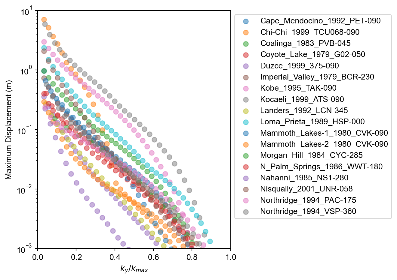
Variation in a single motion’s time history
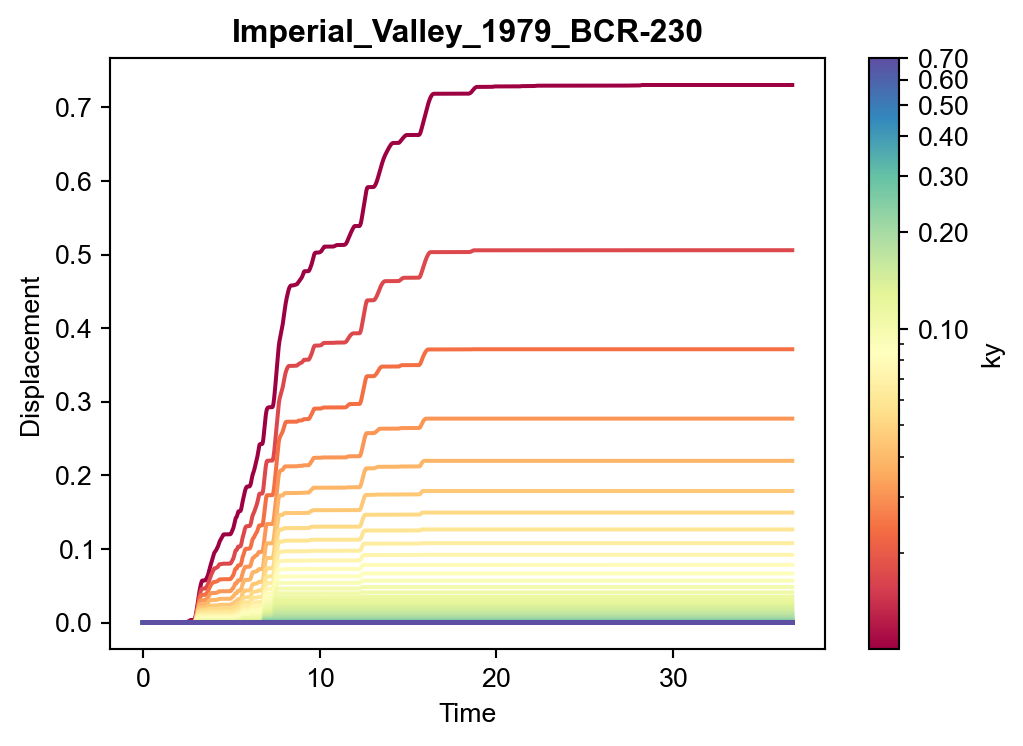
Alternatively, for any given motion, the displacement time histories for different values of \(k_y\) could be of interest. In Figure 2, the results from all the simulations with the Imperial_Valley_1979_BCR-230 motion are shown. Although a different dimension of the data are being shown, the figure is simply pulling from the the results dataframe used in Figure 1.
Code
import matplotlib.cm as cm
from matplotlib.colors import LogNorm

motion = "Imperial_Valley_1979_BCR-230"

plt.close('all')

# Create a figure and axes
fig, ax = plt.subplots(figsize=(6, 4))

# Create a color map
cmap = plt.colormaps['Spectral']#cm.get_cmap('viridis')
norm = LogNorm(df['ky'].min(), df['ky'].max())

dt = df[df["motion"]==motion].iloc[0]['dt']
npts = df[df["motion"]==motion].iloc[0]['disp'].shape[0]
time = np.linspace(0, dt*npts, npts)

for index, row in df[df["motion"]==motion].iterrows():
    color = cmap(norm(row['ky']))
    ax.plot(time, row['disp'], color=color)

# Add a color bar
sm = cm.ScalarMappable(cmap=cmap, norm=norm)
sm.set_array([])
cbar = fig.colorbar(sm, ax=ax, label='ky')

# Set the colorbar ticks and labels
ticks = [0.1, 0.2, 0.3, 0.4, 0.5, 0.6, 0.7]
cbar.set_ticks(ticks)
cbar.set_ticklabels([f'{tick:.2f}' for tick in ticks])

# Set the x-axis and y-axis labels
ax.set_xlabel('Time')
ax.set_ylabel('Displacement')
ax.set_title(motion)
plt.show()