import pyslammer as slam
import numpy as np
import matplotlib.pyplot as pltRigid and Flexible Anlysis
This notebook shows an example use case of pyslammer for running rigid, decoupled, and coupled sliding block analyses.
The next steps assume you’ve already installed pySLAMMER from PYPI. See the quickstart guide for installation instructions.
First, import pySLAMMER and a couple other helpful packages
Next define the ground motion to use in the analysis. For this example, we will use one of pySLAMMER’s built in ground motions from the 1995 Kobe earthquake. This creates a ground motion object with accel and dt attributes with the acceleration array and timestep, respectively.
record_name = "Kobe_1995_TAK-090"
gm = slam.sample_ground_motions()[record_name]
Rigid block analysis
A rigid block analysis requires at least two input parameters:
ground_motion- the input ground motion object, which contains the name, acceleration signal, and timestepky- the slope’s yield acceleration (in units of g)
These parameters are stored in a dictionary (rigid_inputs) and used as kwarg input to the RigidAnalysis method.
rigid_inputs = {
    "ground_motion": gm,
    "ky": 0.2
}

rigid_result = slam.RigidAnalysis(**rigid_inputs)
Note
Passing the input variables to slam.RigidAnalysis as a dictionary isn’t necessary, it’s just a convenient way to package groups of input variables. The following line would have produced the same result as the previous cell:
rigid_result = slam.RigidAnalysis(ground_motion, 0.2)
Flexible sliding block analysis
The flexible block analyses (decoupled and coupled) require additional input parameters to define the stiffness of the model:
height- the slope height (in meters, by default)vs_slope- the slope shear wave velocity (in meters per second, by default)vs_base- the base shear wave velocity (in meters per second, by default)damp_ratio- the slope damping ratioref_strain- the slope reference strainsoil_model- the dynamic analysis method used (eitherlinear_elasticorequivalent_linear)
These parameters are stored in a dictionary (flexible_inputs) and used as kwargs along with those used in the rigid analysis. The decoupled and coupled analyses are run with the Decoupled and Coupled methods, respectively.
flexible_inputs = {
    "height": 50.0,
    "vs_slope": 600.0,
    "vs_base": 600.0,
    "damp_ratio": 0.05,
    "ref_strain": 0.0005,
    "soil_model": "equivalent_linear"
}

decoupled_result = slam.Decoupled(**rigid_inputs,**flexible_inputs)
decoupled_result._compile_attributes()
coupled_result = slam.Coupled(**rigid_inputs,**flexible_inputs)
coupled_result._compile_attributes()
Comparison of analysis methods
A simple plot comparing the block displacements with time can be generated by accessing the .sliding_disp attribute of each analysis result.
Code
# Some extra stuff to make the pplt.figure(figsize=(10, 6))
time = np.arange(0, len(gm.accel) * gm.dt, gm.dt)
# Plot block displacement vs time for each analysis method
plt.plot(time, rigid_result.sliding_disp, label='Rigid Analysis')
plt.plot(time, decoupled_result.sliding_disp, label='Decoupled Analysis')
plt.plot(time, coupled_result.sliding_disp, label='Coupled Analysis')
summary_text = f"ky: {rigid_result.ky / slam.G_EARTH:.2f}g | Motion: {rigid_result.motion_name} (PGA: {max(abs(rigid_result.a_in)):.2f}g)"
plt.suptitle(summary_text, fontsize=10, y=0.98)
# Add labels and legend
plt.xlabel('Time (s)')
plt.ylabel('Block Displacement (m)')
# plt.title(f'Block Displacement with Different Analysis Methods\n for {record_name}')
plt.legend()
plt.grid(True)
# Show the plot
plt.show()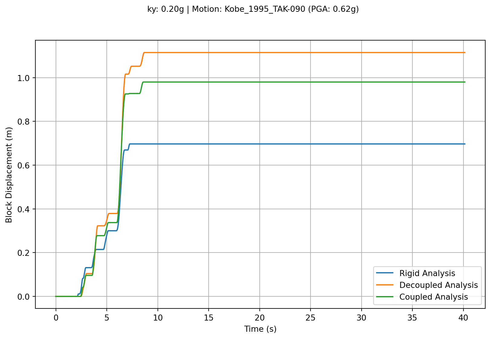
Inherited plotting
Since all of these are instances of classes that have SlidingBlockAnalysis as their parent class, they all inherit the SlidingBlockAnalysis.sliding_block_plot method. Calling the plotting method on each result object produces a concise plot of the analysis. By inspection of the Figure 1, we can see that all the sliding occurs in the first 10 seconds or so of this particular analysis. The plotting method accepts an optional parameter to focus on the time range of interest which will help show some of the differences in the analysis methods.
When we call sliding_block_plot() from rigid_result, the plot shows the familiar features of a traditional “Newmark-like” sliding block analysis.
times = [0,15]
rigid_fig = rigid_result.sliding_block_plot(time_range=times)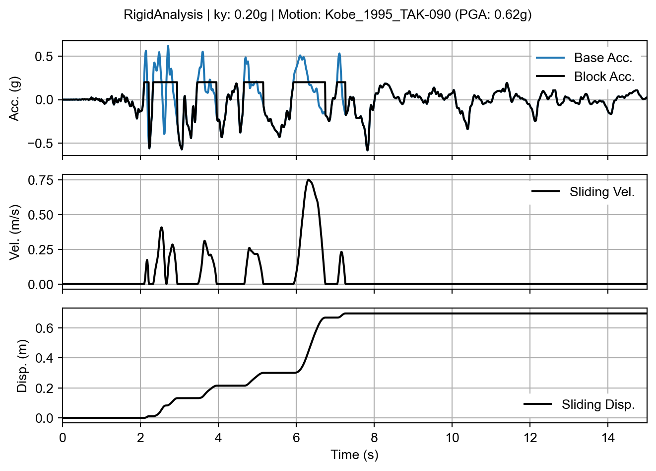
sliding_block_plot() method on the rigid analysis result.
With the decoupled results, the sliding_block_plot() method automatically recognizes the need to display the input motion and the “base” motion as separate arrays. The input acceleration is the motion before the dynamic response of the slope was calculated. The “base” acceleration is the acceleration of the ground beneath the sliding block, which is an output of the slope dynamic response calculation. If we ignore the input acceleration, the base and block acceleration signals look exactly like a rigid analysis result (which is expected because the second half of the decoupled analysis uses rigid sliding assumptions).
decoupled_fig = decoupled_result.sliding_block_plot(time_range=times)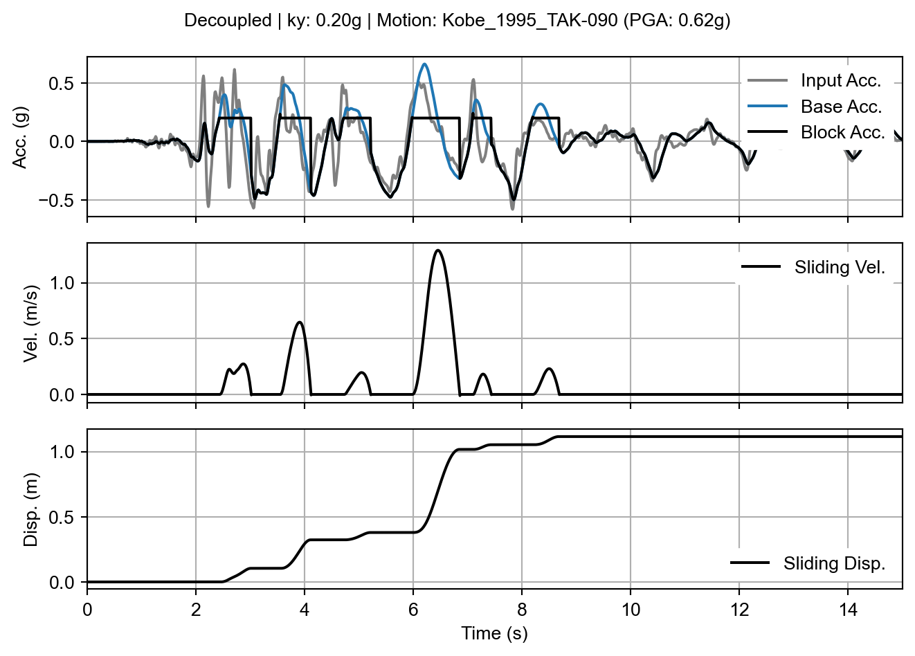
sliding_block_plot() method on the decoupled analysis result.
With the coupled result, we see the differences from the decoupled analysis assumption manifested in the acceleration signals. First, the block acceleration signal no longer shows the distinct plateau of the yield acceleration during sliding events. This is because the dynamic response of the sliding mass continues to be calculated during sliding and the “block acceleration” signal is showing the average acceleration of the whole mass rather than the acceleration at the sliding interface. Second, the base acceleration signal is different than that of the decoupled analysis method during (and very shortly after) sliding because the dynamic response of the slope beneath the failure surface is also affected by sliding. In fact, a close inspection of the stop of sliding times reveals an abrupt jump in the base acceleration as the two masses above and below the sliding surface affect each others’ dynamic response.
coupled_fig = coupled_result.sliding_block_plot(time_range=times)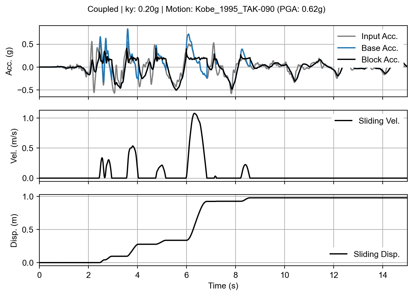
sliding_block_plot() method on the coupled analysis result.